
Database Storage Engines: B-Tree vs. LSM-Tree Architectures
Prerequisites: What a Storage Engine Actually Does
Before comparing architectures, it helps to fix what problem a storage engine solves. Every database splits into two layers: a query layer that parses SQL or CQL and plans execution, and a storage engine underneath that decides how rows physically land on disk and how to find them again. PostgreSQL and MySQL use B-Tree-based engines (InnoDB, in MySQL's case); RocksDB and Cassandra use Log-Structured Merge-Trees, a structure first formalized by Patrick O'Neil, Edward Cheng, Dieter Gawlick, and Elizabeth O'Neil in their 1996 Acta Informatica paper. -O'Neil-Cheng/123fc2af8203708f8bd2b6c3e3d6a41dd8f9a30e)
A few concepts recur throughout both architectures and are worth fixing first:
- Write-ahead log (WAL). Before a change is applied to the main data structure, it's appended to a sequential log file. If the process crashes, the log is replayed to recover uncommitted changes. Both B-Trees and LSM-Trees use one — PostgreSQL calls it the WAL, Cassandra calls it the commit log.
- Page. The unit of I/O for disk-based structures, typically 4–16 KB. B-Trees read and write whole pages even to change a few bytes.
- Amplification (write, read, space). Write amplification (WA) is the ratio of bytes physically written to disk versus bytes the application logically asked to write. Read amplification is how many disk reads a single logical query costs. Space amplification is how much extra disk space stale or duplicate data occupies before it's cleaned up. These three trade off against each other — no engine minimizes all three at once.
- Random vs. sequential I/O. Random I/O jumps around the disk; sequential I/O writes or reads contiguous blocks. On spinning disks the gap is enormous (seek time dominates); on SSDs it's smaller but still real, mainly because sequential writes avoid the SSD's internal write amplification from garbage collection.
With that vocabulary in place, the two architectures are really two different answers to the same question: when a write comes in, do you find its correct sorted position immediately (B-Tree), or do you just append it and sort things out later (LSM-Tree)?
B-Tree Architecture: Update in Place
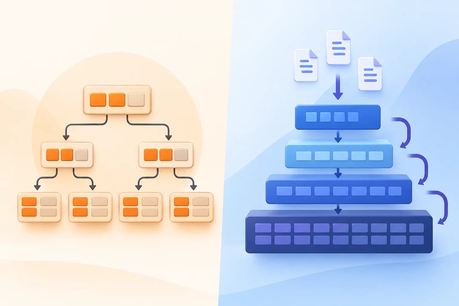
A B-Tree (specifically the B+Tree variant used by nearly every relational database) is a balanced, sorted tree of fixed-size pages. Leaf pages hold the actual row data or pointers to it; internal pages hold routing keys that direct a search down to the right leaf. PostgreSQL's own documentation describes its B-Tree index as "a multi-level tree structure, where each level of the tree can be used as a doubly-linked list of pages," with a single metapage tracking the root.
The defining trait is update-in-place: when you insert or modify a row, the engine locates the exact leaf page where that key belongs, using a top-down tree traversal, and modifies that page directly. MySQL's InnoDB goes further than PostgreSQL by making this the primary storage structure itself — the table's row data lives inside the primary key's B+Tree as a clustered index, so the physical row order follows key order. PostgreSQL instead keeps the B-Tree index separate from the heap file holding row data (a non-clustered/heap-organized approach).
The Write Path
A write to a B-Tree engine follows a predictable sequence: the change is appended to the WAL first (for crash recovery), then the corresponding page is located and modified in the buffer pool (an in-memory cache of pages), and marked dirty. Dirty pages are flushed to disk asynchronously, batched by a background checkpoint process rather than on every write. This is what keeps B-Trees viable for OLTP workloads — the expensive random disk write is deferred and coalesced.
The complication is the page split. B-Tree pages have a fixed capacity. When a page fills up and a new key needs to go in it, the engine splits it into two half-full pages and inserts a pointer to the new page into the parent — which can itself overflow and split, cascading up toward the root. A split that reaches the root is rare but expensive, and it's the mechanism that keeps B-Trees perfectly balanced (all leaves at the same depth) at the cost of occasional extra writes.
Why B-Trees Read Fast
The payoff for all this write-side bookkeeping is a read path with a hard, predictable bound: a point lookup or range scan touches exactly as many pages as the tree is deep, typically 3–4 levels for tables in the tens of millions of rows, because branching factors of several hundred keys per page keep the tree shallow. There's no need to merge results from multiple locations, no duplicate versions of a key to reconcile, no background process competing for I/O bandwidth during the read. This is why B-Trees remain the default for OLTP systems where reads dominate or are latency-sensitive: dashboards, order lookups, user profile fetches.
LSM-Tree Architecture: Append and Compact
The LSM-Tree solves the opposite problem. O'Neil and colleagues designed it explicitly because "standard disk-based index structures such as the B-tree will effectively double the I/O cost of the transaction to maintain an index... in real time" for workloads dominated by high-volume inserts, such as transaction history logs. Instead of finding a key's exact position on every write, the LSM-Tree defers that work and batches it.
The Write Path
A write in an LSM-Tree engine follows this sequence, using RocksDB and Cassandra's implementations as concrete references:
- Write-ahead log. The mutation is appended to a commit log for durability — Cassandra calls it the commit log, RocksDB calls it the WAL.
- Memtable. The write goes into an in-memory sorted structure (often a skip list), with zero disk I/O beyond the log append. Cassandra keeps one active memtable per table.
- Flush. When the memtable hits a size threshold, it's flushed to disk as an immutable, sorted file — an SSTable (Sorted String Table) — in a single sequential write.
- Compaction. Because SSTables are immutable, an update to an existing key doesn't touch the old file — it just gets written as a new entry in a newer SSTable. A background process periodically merges multiple SSTables into fewer, larger ones, discarding superseded versions and deleted (tombstoned) entries. This is a merge-sort over pre-sorted files, which is why it can run on sequential I/O even though it's rewriting large volumes of data.
Cassandra's documentation is blunt about the consequence: "Every write of data in Cassandra is re-written multiple times, known as write amplification, and this adds background I/O to the database workload". That background I/O is compaction working continuously to bound the number of SSTables a read has to check and to reclaim space from obsolete data.
Why Reads Get More Expensive
Because a single key can live in the memtable and in several SSTables simultaneously (with only the newest version valid), a read may have to check multiple locations and merge results by timestamp. Both RocksDB and Cassandra mitigate this with Bloom filters — probabilistic structures that let a read skip an SSTable entirely if it's certain the key isn't present, without doing an actual disk read. This narrows the search but doesn't eliminate the fundamental cost: a cold read in a leveled LSM-Tree can still touch one file per level.
Compaction Strategies and Their Trade-offs
Not all compaction is the same, and the strategy chosen dictates where the LSM-Tree lands on the write/read/space amplification triangle. RocksDB's own wiki documents three production strategies:
| Strategy | Write amplification | Read amplification | Space amplification |
|---|---|---|---|
| Leveled (classic) | High — fanout per level, typically 10–30× | Low — 1–5× | Low — close to 1.1× |
| Universal (tiered) | Low — typically 1–5× | High — 10–50× | Higher — 1.5–2× |
| FIFO | Minimal — ~1× (no rewrites) | Bounded by files in window | ~1× over the window |
Leveled compaction organizes the tree into levels of increasing size, each roughly 10× the previous (the "fanout" or size ratio, T). Merging Ln-1 into Ln rewrites everything in Ln that overlaps the incoming keys — RocksDB's wiki states the per-level write amplification "is equal to the fanout in the worst case," so with a fanout of 10 and 5–6 levels, worst-case cumulative write amplification lands in the 10–30× range commonly cited for production leveled compaction. Universal (tiered) compaction instead merges whole sorted runs without rewriting lower levels on every pass, cutting per-level write amplification to roughly 1×, but it lets more sorted runs accumulate, which is why reads and transient space usage suffer. Cassandra offers both as pluggable strategies — SizeTieredCompactionStrategy for write-heavy workloads, LeveledCompactionStrategy for read-heavy ones — which is a direct acknowledgment that the choice is a workload-specific trade, not a solved problem.
Calculating Write Amplification
Write amplification is defined the same way regardless of engine: physical bytes written to storage divided by logical bytes the application asked to write. The arithmetic differs sharply by structure.
B-Tree Write Amplification
A single-row update generates at minimum two physical writes: the WAL record and the eventual dirty-page flush, giving a floor of roughly 2×. The bigger driver is the mismatch between row size and page size. If a page is 8 KB and a row is 200 bytes, updating that one row still means flushing the entire 8 KB page — an effective byte-level amplification of page_size / row_size, which for small scattered updates against a large table can reach 10–100× before any page-split overhead is even counted. Page splits add a further 2–3 writes when they cascade to a parent. In practice, well-batched sequential inserts stay close to the 2–4× floor, while random-key updates against a large table push toward the higher end — sometimes matching or exceeding an LSM-Tree's amplification, which contradicts the common assumption that B-Trees are always cheaper to write to.
LSM-Tree Write Amplification
The standard model for leveled compaction: for a size ratio (fanout) T between adjacent levels and L levels total, cumulative write amplification is bounded by roughly T × L in the worst case. With T=10 and L=6, that's 60× — consistent with the VLDB paper's observation that write amplification "can be as high as 40× in state-of-the-art LSM-based data stores". In practice, RocksDB's leveled compaction tends to run lower than the worst-case bound because compaction is "some-to-some" (only overlapping key ranges are merged) rather than "all-to-all" as in the original 1996 paper, which is why real deployments commonly report 10–30× rather than the full T×L ceiling.
The key structural difference is when the cost is paid. A B-Tree pays its amplification synchronously, in the foreground, at the moment of the write. An LSM-Tree pays its (larger) amplification asynchronously, in the background, via compaction threads that can be rate-limited, scheduled during low-traffic windows, or run on separate I/O channels — which is why LSM-Trees can sustain higher raw write throughput despite a higher total amplification number: the client-facing write only pays for the memtable and WAL append, not the eventual compaction.
Choosing Between Them
| Dimension | B-Tree (PostgreSQL, InnoDB/MySQL) | LSM-Tree (RocksDB, Cassandra) |
|---|---|---|
| Update mechanism | In-place, on the exact page | Append-only; old versions superseded, not overwritten |
| Write I/O pattern | Random (page-level) | Sequential (memtable flush, compaction merge) |
| Typical write amplification | 2–4× for batched writes; 10–100× for scattered small updates | 10–30× (leveled); 1–5× (tiered/universal) |
| Read path | Deterministic tree descent, 3–4 page reads | May check memtable plus multiple SSTables, mitigated by Bloom filters |
| Background overhead | Checkpointing, page flushes | Continuous compaction competing for I/O and CPU |
| Best suited for | Read-heavy or latency-sensitive OLTP, ad hoc range queries | High-throughput ingest, time-series, logging, write-heavy key-value workloads |
The decision in practice comes down to which cost the workload can absorb. A system logging sensor readings, financial transaction history, or event streams generates continuous high-volume inserts with few random-point reads — exactly the profile O'Neil's team designed the LSM-Tree for in 1996, citing account-history tables as the motivating case. A system serving a web application's primary transactional data, where every user request needs a fast, predictable lookup and updates are comparatively infrequent, is what B-Trees were built to serve well, and it's why PostgreSQL and MySQL — general-purpose relational engines — default to them. -O'Neil-Cheng/123fc2af8203708f8bd2b6c3e3d6a41dd8f9a30e)
Neither architecture is a free lunch on amplification; each just moves the cost to a different place: the B-Tree pays in random I/O at write time, the LSM-Tree pays in background rewrite volume during compaction. Understanding which bill your workload will actually incur — not which structure sounds more modern — is the real basis for the choice.