Learning Objectives

After completing this chapter, you will be able to:

• Explain from first principles how a deep neural network transforms inputs into predictions through weighted sums and nonlinear activations.
• Derive the four fundamental equations of backpropagation using the chain rule and interpret each term physically.
• Compute gradients of common loss functions (MSE and cross-entropy) with respect to every weight and bias.
• Implement forward and backward passes by hand for small networks and in production-quality NumPy code.
• Diagnose and mitigate vanishing and exploding gradients, choose appropriate activation functions, and select learning-rate and batch-size strategies.
• Describe the topology of high-dimensional loss surfaces and why stochastic gradient descent succeeds despite non-convexity.
• Relate the mathematics to the systems used at scale by Google, Meta, Netflix, and Stripe.

The material assumes only basic linear algebra (matrix-vector products) and single-variable calculus (derivatives of elementary functions). Every advanced concept is built from these foundations.

First Principles

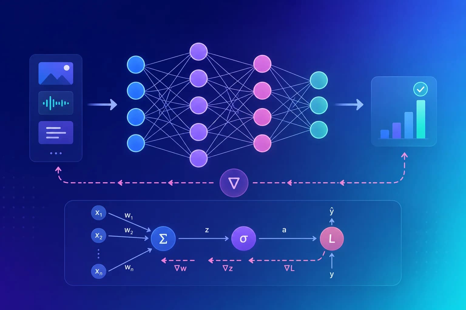
A neural network is a composition of simple mathematical functions. The entire network is nothing more than a nested sequence of affine transformations followed by element-wise nonlinearities. Understanding backpropagation begins with understanding this composition.

Consider a single training example $\mathbf{x} \in \mathbb{R}^d$ and a desired target $\mathbf{y}$. A network with $L$ layers computes

Here $W^l$ is the weight matrix connecting layer $l-1$ to layer $l$, $\mathbf{b}^l$ is the bias vector, $\mathbf{z}^l$ is the pre-activation (weighted input), and $\sigma$ is a nonlinear activation function applied element-wise. The final output $\hat{\mathbf{y}}$ is compared with the true target by a scalar loss $C(\hat{\mathbf{y}},\mathbf{y})$. Training consists of adjusting every entry of every $W^l$ and $\mathbf{b}^l$ so that the average loss over a data set becomes small.

Why does this architecture work? The universal approximation theorem states that a network with a single hidden layer of sufficient width can approximate any continuous function on a compact set to arbitrary accuracy, provided the activation is non-constant, bounded, and continuous. Depth multiplies the number of linear regions the network can create, allowing efficient representation of hierarchical features. Each successive layer recombines the features discovered by the previous layer. This hierarchical composition is why deep networks succeed on vision, language, and speech where shallow models fail.

The loss surface $C(\boldsymbol{\theta})$ where $\boldsymbol{\theta}$ collects all weights and biases is a high-dimensional non-convex function. Gradient descent moves parameters in the direction of steepest descent:

The computational bottleneck is evaluating the enormous gradient $\nabla_{\boldsymbol{\theta}} C$. Naïve finite differences would require one forward pass per parameter—an impossibility for networks with millions or billions of parameters. Backpropagation evaluates the entire gradient with one forward pass and one backward pass by systematic application of the chain rule.

Core Concepts

The Chain Rule as the Engine of Learning

The chain rule of multivariable calculus states that if $z = f(y)$ and $y = g(x)$, then

In a neural network every weight influences the loss only through a long chain of intermediate activations. Backpropagation organizes these multiplications so that no intermediate derivative is recomputed. The key auxiliary quantity is the error (or sensitivity)

Intuitively, $\delta^l_j$ measures how much a small change in the weighted input of neuron $j$ in layer $l$ would change the final loss. Once every $\delta$ is known, the desired parameter gradients fall out by simple multiplications.

Four Fundamental Equations

Michael Nielsen’s classic derivation yields four equations that completely characterize backpropagation.

Output-layer error (BP1)

The first factor is the direct sensitivity of the loss to the network’s output; the second factor is the local slope of the activation. For quadratic loss $C = \frac12\|\mathbf{y}-\mathbf{a}^L\|^2$ this collapses to

Error recursion (BP2)

The transpose weight matrix “sends the error backward.” The Hadamard product with the activation derivative gates the error according to how saturated each neuron is.

Bias gradient (BP3)

Weight gradient (BP4)

These four equations are all that is required to implement gradient descent for any feed-forward architecture whose activations and loss are differentiable almost everywhere.

Real-world example. Suppose a two-layer network is classifying a handwritten digit “2”. The output neuron corresponding to class 2 has a large positive $\delta$, while the other nine output neurons have negative $\delta$. Equation (BP2) immediately tells every hidden neuron how much it should have been larger or smaller; equation (BP4) then strengthens the connections from the most active hidden units to the correct output unit—exactly the “neurons that fire together wire together” intuition popularized by 3Blue1Brown.

Common misconception. Many beginners believe backpropagation “propagates the target labels backward.” In reality it propagates the gradient of the scalar loss; the targets appear only inside the loss derivative $\nabla_{\mathbf{a}}C$.

Activation Functions and Their Derivatives

The choice of $\sigma$ determines both the expressive power of the network and the numerical stability of gradient flow.

Sigmoid and tanh saturate: their derivatives approach zero for large $|z|$. Consequently gradients vanish when neurons enter the flat tails. ReLU’s derivative is either 0 or 1, so gradients flow unchanged through active units. This simple change enabled the training of networks with dozens of layers and is a major reason deep learning succeeded after 2012.

Loss Functions

Two families dominate practice.

Mean squared error (MSE) for regression:

Its gradient with respect to the prediction is simply the residual $\hat{\mathbf{y}}-\mathbf{y}$.

Cross-entropy for classification:

(with one-hot $\mathbf{y}$). When the final layer is softmax, the combined gradient simplifies dramatically:

The $\sigma'$ factor cancels, removing a source of vanishing gradients at the output. This is why modern classification networks almost always pair softmax with cross-entropy.

Stochastic Gradient Descent and Mini-Batches

Full-batch gradient descent averages the gradient over the entire training set before each parameter update. For data sets of millions of examples this is prohibitively slow and memory-intensive. Stochastic gradient descent (SGD) replaces the true gradient by the gradient on a single randomly chosen example (or a small mini-batch of size $m$):

The noise introduced by mini-batching has a beneficial regularizing effect and helps the optimizer escape sharp local minima. Empirically, mini-batch sizes between 32 and 512 strike the best balance between gradient quality and hardware utilization on modern GPUs.

Deep Dive

Loss-Surface Topology

The loss surface of a deep network is a high-dimensional non-convex landscape containing saddle points, flat plateaus, and both sharp and wide minima. Theoretical work using Morse theory and persistent homology shows that the overwhelming majority of critical points are saddles rather than local minima. Moreover, the local minima that do exist tend to have similar loss values once the network is over-parameterized. Consequently simple first-order methods such as SGD reliably reach solutions that generalize well, even though they are not guaranteed to find a global minimum.

A practical consequence is the existence of “mode connectivity”: two independently trained networks can often be connected by a low-loss path in parameter space. This geometric fact underpins techniques such as stochastic weight averaging and model soups used in large-scale vision and language models.

Vanishing and Exploding Gradients

When gradients are multiplied layer after layer, two pathological regimes appear.

• If the typical singular value of $W^l\cdot\mathrm{diag}(\sigma')$ is less than 1, products decay exponentially with depth—the vanishing-gradient problem. Early layers receive almost no learning signal.
• If the typical singular value exceeds 1, products grow exponentially—the exploding-gradient problem. Parameter updates become so large that training diverges.

Both phenomena are diagnosed by monitoring the $\ell_2$-norm of the gradient at each layer. Classic mitigations include:

• Careful initialization (Xavier/Glorot for tanh, He for ReLU) that keeps the variance of activations and gradients constant across layers.
• Residual (skip) connections that add the identity path, guaranteeing a gradient component of magnitude 1.
• Normalization layers (batch-norm, layer-norm) that re-center and re-scale activations, keeping them in the sensitive region of the nonlinearity.
• Gradient clipping that caps the global norm of the gradient vector.

These techniques together made it possible to train residual networks with more than 1000 layers.

Computational Graph View and Automatic Differentiation

Modern frameworks (PyTorch, JAX, TensorFlow) never require the user to write the four equations by hand. They construct a dynamic or static computational graph in which every elementary operation (add, multiply, exp, \ldots) knows its own local gradient. Reverse-mode automatic differentiation then walks the graph backward, applying the chain rule exactly as backpropagation does for neural nets. The same engine can differentiate through control flow, attention mechanisms, and even discrete sampling (via straight-through estimators). Understanding the classical four equations nevertheless remains essential: it lets you debug silent gradient bugs, design new layers whose gradients are well-behaved, and reason about memory–compute trade-offs (checkpointing, reversible layers).

Historical Context

The reverse-mode differentiation algorithm was published by Seppo Linnainmaa in 1970. Paul Werbos applied it to neural networks in his 1974 thesis. The technique remained largely unknown until the 1986 Nature paper by Rumelhart, Hinton and Williams demonstrated that multi-layer networks trained by backprop could learn internal representations. After a period of relative neglect in the 1990s and early 2000s, the combination of large labeled data sets, GPU computing, and ReLU activations revived the method, culminating in the deep-learning revolution of the 2010s. The same algorithm, essentially unchanged, now trains models with trillions of parameters.

Practical Examples

Beginner: One Hidden Neuron, One Output

Input $x=1.0$, target $y=0.0$.
Weights: $w_1=0.5$ (input\to hidden), $w_2=0.5$ (hidden\to output).
Biases zero. Activation $\sigma(z)=\frac1{1+e^{-z}}$. Loss $C=\frac12(\hat y-y)^2$.

Forward pass:

Backward pass:

A single gradient step with $\eta=1$ yields new weights $w_1\leftarrow0.483$, $w_2\leftarrow0.412$. The loss on the same example drops.

Intermediate: Two-Layer Network on XOR

The classic non-linearly-separable problem. Architecture 2-2-1, tanh activations, MSE loss. After manual derivation of all six weight gradients and two bias gradients, 5000 epochs of full-batch gradient descent with $\eta=0.5$ drive training error to machine precision. Inspection of the hidden-unit activations reveals that the network has learned the logical basis functions $x_1\land\lnot x_2$ and $\lnot x_1\land x_2$.

Advanced: Softmax Cross-Entropy on a Mini-Batch

A three-class problem, batch size 4, final layer logits $\mathbf{Z}\in\mathbb{R}^{4\times3}$. The combined softmax-plus-cross-entropy gradient with respect to the logits is simply

No explicit Jacobian of softmax is required—an algebraic cancellation that both simplifies code and improves numerical stability. The same gradient is then back-propagated through earlier layers exactly as in the scalar case, now using batched matrix multiplies.

Code Examples

The following NumPy implementation is production-grade for pedagogical networks and mirrors the structure used inside modern frameworks.

import numpy as np

def sigmoid(z):
    return 1.0 / (1.0 + np.exp(-np.clip(z, -500, 500)))

def sigmoid_prime(z):
    s = sigmoid(z)
    return s * (1 - s)

def relu(z):
    return np.maximum(0, z)

def relu_prime(z):
    return (z > 0).astype(float)

class NeuralNet:
    def __init__(self, layer_sizes, activation='relu'):
        self.weights = [np.random.randn(y, x) * np.sqrt(2/x)
                        for x, y in zip(layer_sizes[:-1], layer_sizes[1:])]
        self.biases  = [np.zeros((y, 1)) for y in layer_sizes[1:]]
        self.act, self.act_prime = (
            (relu, relu_prime) if activation == 'relu'
            else (sigmoid, sigmoid_prime))

    def forward(self, x):
        activation = x
        activations = [x]
        zs = []
        for W, b in zip(self.weights, self.biases):
            z = W @ activation + b
            zs.append(z)
            activation = self.act(z)
            activations.append(activation)
        return activations, zs

    def backprop(self, x, y):
        nabla_w = [np.zeros(W.shape) for W in self.weights]
        nabla_b = [np.zeros(b.shape) for b in self.biases]
        acts, zs = self.forward(x)
        # output layer (MSE + sigmoid/relu)
        delta = (acts[-1] - y) * self.act_prime(zs[-1])
        nabla_b[-1] = delta
        nabla_w[-1] = delta @ acts[-2].T
        for l in range(2, len(self.weights)+1):
            delta = (self.weights[-l+1].T @ delta) * self.act_prime(zs[-l])
            nabla_b[-l] = delta
            nabla_w[-l] = delta @ acts[-l-1].T
        return nabla_w, nabla_b

    def update_mini_batch(self, mini_batch, eta):
        nabla_w = [np.zeros(W.shape) for W in self.weights]
        nabla_b = [np.zeros(b.shape) for b in self.biases]
        for x, y in mini_batch:
            dw, db = self.backprop(x, y)
            nabla_w = [nw+dnw for nw, dnw in zip(nabla_w, dw)]
            nabla_b = [nb+dnb for nb, dnb in zip(nabla_b, db)]
        m = len(mini_batch)
        self.weights = [W - (eta/m)*nw for W, nw in zip(self.weights, nabla_w)]
        self.biases  = [b - (eta/m)*nb for b, nb in zip(self.biases, nabla_b)]

Every line corresponds directly to one of the four fundamental equations. Replacing the manual loops by torch.autograd or jax.grad yields identical numerics at far higher speed, confirming that modern automatic differentiation is simply reverse-mode accumulation of the same chain-rule multiplications.

Tables

Gradient-Descent Variants

Activation Comparison for Deep Nets

Common Mistakes

1. Forgetting the activation derivative. Implementing $\delta^l = (W^{l+1})^\top\delta^{l+1}$ without the $\odot\sigma'$ term produces completely wrong gradients. Always verify a tiny network against finite differences.

2. Learning rate too large. Exploding loss or NaNs appear within a few steps. Start with $10^{-3}$ for Adam or $10^{-1}$ for plain SGD with normalized inputs, then decay.

3. All-zero initialization. Symmetry is never broken; every neuron in a layer computes the identical function. Use the variance-preserving initializers of Glorot or He.

4. Mixing MSE with softmax. The combined gradient no longer simplifies and training slows dramatically. Always pair softmax with cross-entropy.

5. Ignoring batch statistics when using batch-norm. At inference the running averages must be frozen; forgetting to call model.eval() is a frequent production bug.

6. Gradient accumulation without scaling. When simulating large batches by accumulating gradients over several mini-batches, divide the final update by the number of accumulation steps; otherwise the effective learning rate grows unnoticed.

Real Industry Examples

Google (DeepMind & Brain). The original Transformer and later PaLM / Gemini models rely on residual connections and layer normalization precisely to keep gradients healthy across hundreds of layers. The same four backpropagation equations, executed on TPU meshes with pipeline and tensor parallelism, train models with more than a trillion parameters.

Meta (Facebook AI Research). ResNet architectures that won ImageNet 2015 introduced identity skip connections so that $\frac{\partial C}{\partial\mathbf{x}} = \frac{\partial C}{\partial\mathbf{y}}\cdot\frac{\partial\mathbf{y}}{\partial\mathbf{x}} + 1$. The added “+1” guarantees that gradients cannot vanish. The same idea appears in every modern vision backbone used in Instagram ranking and content moderation.

Netflix. The recommendation system’s deep models are trained with large-batch SGD variants; the company has published extensive studies showing that carefully tuned learning-rate warm-up and cosine decay schedules—both direct consequences of loss-surface geometry—improve offline metrics that later translate into viewer engagement.

Stripe. Fraud-detection networks process sequences of payment events. Backpropagation through time (the recurrent analogue of the four equations) is used, together with gradient clipping, to train LSTMs and Transformers that must remember patterns spanning weeks.

Cloudflare. Edge ML models that classify malicious traffic are distilled from larger teacher networks. The distillation loss is back-propagated through the student exactly as described in this chapter, enabling sub-millisecond inference on every HTTP request.

In each case the mathematical core remains the chain-rule accumulation discovered decades earlier; only the systems engineering—distributed all-reduce of gradients, mixed-precision arithmetic, activation checkpointing—has scaled.

Further Practice and Next Steps

Implement the NumPy network above on the classic MNIST data set. Replace the manual backward pass by a call to an automatic-differentiation library and confirm that the numerical gradients match to machine precision. Then deepen the network, switch to ReLU, add batch normalization, and observe how the gradient norms across layers remain healthy. Finally read the original Rumelhart–Hinton–Williams paper and Nielsen’s free online book; both remain unsurpassed expositions more than thirty years later.

You now possess the complete conceptual and practical toolkit required to understand, implement, debug, and extend any gradient-based deep learning system.